AI with Python – Supervised Learning: Classification

---

In this chapter, we will focus on implementing supervised learning − classification.

The classification technique or model attempts to get some conclusion from observed values. In classification problem, we have the categorized output such as “Black” or “white” or “Teaching” and “Non-Teaching”. While building the classification model, we need to have training dataset that contains data points and the corresponding labels. For example, if we want to check whether the image is of a car or not. For checking this, we will build a training dataset having the two classes related to “car” and “no car”. Then we need to train the model by using the training samples. The classification models are mainly used in face recognition, spam identification, etc.

Steps for Building a Classifier in Python

For building a classifier in Python, we are going to use Python 3 and Scikit-learn which is a tool for machine learning. Follow these steps to build a classifier in Python −

Step 1 − Import Scikit-learn

This would be very first step for building a classifier in Python. In this step, we will install a Python package called Scikit-learn which is one of the best machine learning modules in Python. The following command will help us import the package −

Import Sklearn

Step 2 − Import Scikit-learn’s dataset

In this step, we can begin working with the dataset for our machine learning model. Here, we are going to use the Breast Cancer Wisconsin Diagnostic Database. The dataset includes various information about breast cancer tumors, as well as classification labels of malignant or benign. The dataset has 569 instances, or data, on 569 tumors and includes information on 30 attributes, or features, such as the radius of the tumor, texture, smoothness, and area. With the help of the following command, we can import the Scikit-learn’s breast cancer dataset −

from sklearn.datasets import load_breast_cancer

Now, the following command will load the dataset.

data = load_breast_cancer()

Following is a list of important dictionary keys −

• Classification label names(target_names)
• The actual labels(target)
• The attribute/feature names(feature_names)
• The attribute (data)

Now, with the help of the following command, we can create new variables for each important set of information and assign the data. In other words, we can organize the data with the following commands −

label_names = data['target_names']
labels = data['target']
feature_names = data['feature_names']
features = data['data']

Now, to make it clearer we can print the class labels, the first data instance’s label, our feature names and the feature’s value with the help of the following commands −

print(label_names)

The above command will print the class names which are malignant and benign respectively. It is shown as the output below −

['malignant' 'benign']

Now, the command below will show that they are mapped to binary values 0 and 1. Here 0 represents malignant cancer and 1 represents benign cancer. You will receive the following output −

print(labels[0])
0

The two commands given below will produce the feature names and feature values.

print(feature_names[0])
mean radius
print(features[0])
[ 1.79900000e+01 1.03800000e+01 1.22800000e+02 1.00100000e+03
  1.18400000e-01 2.77600000e-01 3.00100000e-01 1.47100000e-01
  2.41900000e-01 7.87100000e-02 1.09500000e+00 9.05300000e-01
  8.58900000e+00 1.53400000e+02 6.39900000e-03 4.90400000e-02
  5.37300000e-02 1.58700000e-02 3.00300000e-02 6.19300000e-03
  2.53800000e+01 1.73300000e+01 1.84600000e+02 2.01900000e+03
  1.62200000e-01 6.65600000e-01 7.11900000e-01 2.65400000e-01
  4.60100000e-01 1.18900000e-01]

From the above output, we can see that the first data instance is a malignant tumor the radius of which is 1.7990000e+01.

Step 3 − Organizing data into sets

In this step, we will divide our data into two parts namely a training set and a test set. Splitting the data into these sets is very important because we have to test our model on the unseen data. To split the data into sets, sklearn has a function called the train_test_split() function. With the help of the following commands, we can split the data in these sets −

from sklearn.model_selection import train_test_split

The above command will import the train_test_split function from sklearn and the command below will split the data into training and test data. In the example given below, we are using 40 % of the data for testing and the remaining data would be used for training the model.

train, test, train_labels, test_labels = train_test_split(features,labels,test_size = 0.40, random_state = 42)

Step 4 − Building the model

In this step, we will be building our model. We are going to use Naïve Bayes algorithm for building the model. Following commands can be used to build the model −

from sklearn.naive_bayes import GaussianNB

The above command will import the GaussianNB module. Now, the following command will help you initialize the model.

gnb = GaussianNB()

We will train the model by fitting it to the data by using gnb.fit().

model = gnb.fit(train, train_labels)

Step 5 − Evaluating the model and its accuracy

In this step, we are going to evaluate the model by making predictions on our test data. Then we will find out its accuracy also. For making predictions, we will use the predict() function. The following command will help you do this −

preds = gnb.predict(test)
print(preds)

[1 0 0 1 1 0 0 0 1 1 1 0 1 0 1 0 1 1 1 0 1 1 0 1 1 1 1 1 1
 0 1 1 1 1 1 1 0 1 0 1 1 0 1 1 1 1 1 1 1 1 0 0 1 1 1 1 1 0 
 0 1 1 0 0 1 1 1 0 0 1 1 0 0 1 0 1 1 1 1 1 1 0 1 1 0 0 0 0 
 0 1 1 1 1 1 1 1 1 0 0 1 0 0 1 0 0 1 1 1 0 1 1 0 1 1 0 0 0 
 1 1 1 0 0 1 1 0 1 0 0 1 1 0 0 0 1 1 1 0 1 1 0 0 1 0 1 1 0 
 1 0 0 1 1 1 1 1 1 1 0 0 1 1 1 1 1 1 1 1 1 1 1 1 0 1 1 1 0 
 1 1 0 1 1 1 1 1 1 0 0 0 1 1 0 1 0 1 1 1 1 0 1 1 0 1 1 1 0 
 1 0 0 1 1 1 1 1 1 1 1 0 1 1 1 1 1 0 1 0 0 1 1 0 1]

The above series of 0s and 1s are the predicted values for the tumor classes – malignant and benign.

Now, by comparing the two arrays namely test_labels and preds, we can find out the accuracy of our model. We are going to use the accuracy_score() function to determine the accuracy. Consider the following command for this −

from sklearn.metrics import accuracy_score
print(accuracy_score(test_labels,preds))
0.951754385965

The result shows that the NaïveBayes classifier is 95.17% accurate.

In this way, with the help of the above steps we can build our classifier in Python.

Building Classifier in Python

In this section, we will learn how to build a classifier in Python.

Naïve Bayes Classifier

Naïve Bayes is a classification technique used to build classifier using the Bayes theorem. The assumption is that the predictors are independent. In simple words, it assumes that the presence of a particular feature in a class is unrelated to the presence of any other feature. For building Naïve Bayes classifier we need to use the python library called scikit learn. There are three types of Naïve Bayes models named Gaussian, Multinomial and Bernoulli under scikit learn package.

To build a Naïve Bayes machine learning classifier model, we need the following &minus

Dataset

We are going to use the dataset named Breast Cancer Wisconsin Diagnostic Database. The dataset includes various information about breast cancer tumors, as well as classification labels of malignant or benign. The dataset has 569 instances, or data, on 569 tumors and includes information on 30 attributes, or features, such as the radius of the tumor, texture, smoothness, and area. We can import this dataset from sklearn package.

Naïve Bayes Model

For building Naïve Bayes classifier, we need a Naïve Bayes model. As told earlier, there are three types of Naïve Bayes models named Gaussian, Multinomial and Bernoulli under scikit learn package. Here, in the following example we are going to use the Gaussian Naïve Bayes model.

By using the above, we are going to build a Naïve Bayes machine learning model to use the tumor information to predict whether or not a tumor is malignant or benign.

To begin with, we need to install the sklearn module. It can be done with the help of the following command −

Import Sklearn

Now, we need to import the dataset named Breast Cancer Wisconsin Diagnostic Database.

from sklearn.datasets import load_breast_cancer

Now, the following command will load the dataset.

data = load_breast_cancer()

The data can be organized as follows −

label_names = data['target_names']
labels = data['target']
feature_names = data['feature_names']
features = data['data']

Now, to make it clearer we can print the class labels, the first data instance’s label, our feature names and the feature’s value with the help of following commands −

print(label_names)

The above command will print the class names which are malignant and benign respectively. It is shown as the output below −

['malignant' 'benign']

Now, the command given below will show that they are mapped to binary values 0 and 1. Here 0 represents malignant cancer and 1 represents benign cancer. It is shown as the output below −

print(labels[0])
0

The following two commands will produce the feature names and feature values.

print(feature_names[0])
mean radius
print(features[0])

[ 1.79900000e+01 1.03800000e+01 1.22800000e+02 1.00100000e+03
  1.18400000e-01 2.77600000e-01 3.00100000e-01 1.47100000e-01
  2.41900000e-01 7.87100000e-02 1.09500000e+00 9.05300000e-01
  8.58900000e+00 1.53400000e+02 6.39900000e-03 4.90400000e-02
  5.37300000e-02 1.58700000e-02 3.00300000e-02 6.19300000e-03
  2.53800000e+01 1.73300000e+01 1.84600000e+02 2.01900000e+03
  1.62200000e-01 6.65600000e-01 7.11900000e-01 2.65400000e-01
  4.60100000e-01 1.18900000e-01]

From the above output, we can see that the first data instance is a malignant tumor the main radius of which is 1.7990000e+01.

For testing our model on unseen data, we need to split our data into training and testing data. It can be done with the help of the following code −

from sklearn.model_selection import train_test_split

The above command will import the train_test_split function from sklearn and the command below will split the data into training and test data. In the below example, we are using 40 % of the data for testing and the remining data would be used for training the model.

train, test, train_labels, test_labels = 
train_test_split(features,labels,test_size = 0.40, random_state = 42)

Now, we are building the model with the following commands −

from sklearn.naive_bayes import GaussianNB

The above command will import the GaussianNB module. Now, with the command given below, we need to initialize the model.

gnb = GaussianNB()

We will train the model by fitting it to the data by using gnb.fit().

model = gnb.fit(train, train_labels)

Now, evaluate the model by making prediction on the test data and it can be done as follows −

preds = gnb.predict(test)
print(preds)

[1 0 0 1 1 0 0 0 1 1 1 0 1 0 1 0 1 1 1 0 1 1 0 1 1 1 1 1 1
 0 1 1 1 1 1 1 0 1 0 1 1 0 1 1 1 1 1 1 1 1 0 0 1 1 1 1 1 0 
 0 1 1 0 0 1 1 1 0 0 1 1 0 0 1 0 1 1 1 1 1 1 0 1 1 0 0 0 0 
 0 1 1 1 1 1 1 1 1 0 0 1 0 0 1 0 0 1 1 1 0 1 1 0 1 1 0 0 0 
 1 1 1 0 0 1 1 0 1 0 0 1 1 0 0 0 1 1 1 0 1 1 0 0 1 0 1 1 0 
 1 0 0 1 1 1 1 1 1 1 0 0 1 1 1 1 1 1 1 1 1 1 1 1 0 1 1 1 0 
 1 1 0 1 1 1 1 1 1 0 0 0 1 1 0 1 0 1 1 1 1 0 1 1 0 1 1 1 0 
 1 0 0 1 1 1 1 1 1 1 1 0 1 1 1 1 1 0 1 0 0 1 1 0 1]

The above series of 0s and 1s are the predicted values for the tumor classes i.e. malignant and benign.

Now, by comparing the two arrays namely test_labels and preds, we can find out the accuracy of our model. We are going to use the accuracy_score() function to determine the accuracy. Consider the following command −

from sklearn.metrics import accuracy_score
print(accuracy_score(test_labels,preds))
0.951754385965

The result shows that NaïveBayes classifier is 95.17% accurate.

That was machine learning classifier based on the Naïve Bayse Gaussian model.

Support Vector Machines (SVM)

Basically, Support vector machine (SVM) is a supervised machine learning algorithm that can be used for both regression and classification. The main concept of SVM is to plot each data item as a point in n-dimensional space with the value of each feature being the value of a particular coordinate. Here n would be the features we would have. Following is a simple graphical representation to understand the concept of SVM −

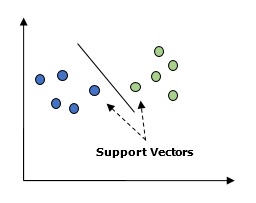
In the above diagram, we have two features. Hence, we first need to plot these two variables in two dimensional space where each point has two co-ordinates, called support vectors. The line splits the data into two different classified groups. This line would be the classifier.

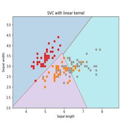
Here, we are going to build an SVM classifier by using scikit-learn and iris dataset. Scikitlearn library has the sklearn.svm module and provides sklearn.svm.svc for classification. The SVM classifier to predict the class of the iris plant based on 4 features are shown below.

Dataset

We will use the iris dataset which contains 3 classes of 50 instances each, where each class refers to a type of iris plant. Each instance has the four features namely sepal length, sepal width, petal length and petal width. The SVM classifier to predict the class of the iris plant based on 4 features is shown below.

Kernel

It is a technique used by SVM. Basically these are the functions which take low-dimensional input space and transform it to a higher dimensional space. It converts non-separable problem to separable problem. The kernel function can be any one among linear, polynomial, rbf and sigmoid. In this example, we will use the linear kernel.

Let us now import the following packages −

import pandas as pd
import numpy as np
from sklearn import svm, datasets
import matplotlib.pyplot as plt

Now, load the input data −

iris = datasets.load_iris()

We are taking first two features −

X = iris.data[:, :2]
y = iris.target

We will plot the support vector machine boundaries with original data. We are creating a mesh to plot.

x_min, x_max = X[:, 0].min() - 1, X[:, 0].max() + 1
y_min, y_max = X[:, 1].min() - 1, X[:, 1].max() + 1
h = (x_max / x_min)/100
xx, yy = np.meshgrid(np.arange(x_min, x_max, h),
np.arange(y_min, y_max, h))
X_plot = np.c_[xx.ravel(), yy.ravel()]

We need to give the value of regularization parameter.

C = 1.0

We need to create the SVM classifier object.

Svc_classifier = svm_classifier.SVC(kernel='linear', 
C=C, decision_function_shape = 'ovr').fit(X, y)
Z = svc_classifier.predict(X_plot)
Z = Z.reshape(xx.shape)
plt.figure(figsize = (15, 5))
plt.subplot(121)
plt.contourf(xx, yy, Z, cmap = plt.cm.tab10, alpha = 0.3)
plt.scatter(X[:, 0], X[:, 1], c = y, cmap = plt.cm.Set1)
plt.xlabel('Sepal length')
plt.ylabel('Sepal width')
plt.xlim(xx.min(), xx.max())
plt.title('SVC with linear kernel')

Logistic Regression

Basically, logistic regression model is one of the members of supervised classification algorithm family. Logistic regression measures the relationship between dependent variables and independent variables by estimating the probabilities using a logistic function.

Here, if we talk about dependent and independent variables then dependent variable is the target class variable we are going to predict and on the other side the independent variables are the features we are going to use to predict the target class.

In logistic regression, estimating the probabilities means to predict the likelihood occurrence of the event. For example, the shop owner would like to predict the customer who entered into the shop will buy the play station (for example) or not. There would be many features of customer − gender, age, etc. which would be observed by the shop keeper to predict the likelihood occurrence, i.e., buying a play station or not. The logistic function is the sigmoid curve that is used to build the function with various parameters.

Prerequisites

Before building the classifier using logistic regression, we need to install the Tkinter package on our system. It can be installed from https://docs.python.org/2/library/tkinter.html.

Now, with the help of the code given below, we can create a classifier using logistic regression −

First, we will import some packages −

import numpy as np
from sklearn import linear_model
import matplotlib.pyplot as plt

Now, we need to define the sample data which can be done as follows −

X = np.array([[2, 4.8], [2.9, 4.7], [2.5, 5], [3.2, 5.5], [6, 5], [7.6, 4],
              [3.2, 0.9], [2.9, 1.9],[2.4, 3.5], [0.5, 3.4], [1, 4], [0.9, 5.9]])
y = np.array([0, 0, 0, 1, 1, 1, 2, 2, 2, 3, 3, 3])

Next, we need to create the logistic regression classifier, which can be done as follows −

Classifier_LR = linear_model.LogisticRegression(solver = 'liblinear', C = 75)

Last but not the least, we need to train this classifier −

Classifier_LR.fit(X, y)

Now, how we can visualize the output? It can be done by creating a function named Logistic_visualize() −

Def Logistic_visualize(Classifier_LR, X, y):
   min_x, max_x = X[:, 0].min() - 1.0, X[:, 0].max() + 1.0
   min_y, max_y = X[:, 1].min() - 1.0, X[:, 1].max() + 1.0

In the above line, we defined the minimum and maximum values X and Y to be used in mesh grid. In addition, we will define the step size for plotting the mesh grid.

mesh_step_size = 0.02

Let us define the mesh grid of X and Y values as follows −

x_vals, y_vals = np.meshgrid(np.arange(min_x, max_x, mesh_step_size),
                 np.arange(min_y, max_y, mesh_step_size))

With the help of following code, we can run the classifier on the mesh grid −

output = classifier.predict(np.c_[x_vals.ravel(), y_vals.ravel()])
output = output.reshape(x_vals.shape)
plt.figure()
plt.pcolormesh(x_vals, y_vals, output, cmap = plt.cm.gray)
 
plt.scatter(X[:, 0], X[:, 1], c = y, s = 75, edgecolors = 'black', 
linewidth=1, cmap = plt.cm.Paired)

The following line of code will specify the boundaries of the plot

plt.xlim(x_vals.min(), x_vals.max())
plt.ylim(y_vals.min(), y_vals.max())
plt.xticks((np.arange(int(X[:, 0].min() - 1), int(X[:, 0].max() + 1), 1.0)))
plt.yticks((np.arange(int(X[:, 1].min() - 1), int(X[:, 1].max() + 1), 1.0)))
plt.show()

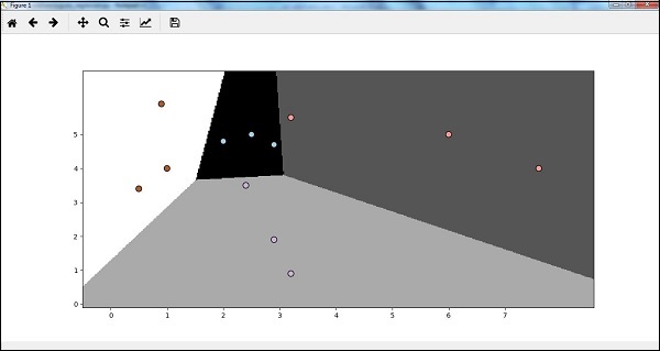
Now, after running the code we will get the following output, logistic regression classifier −

Decision Tree Classifier

A decision tree is basically a binary tree flowchart where each node splits a group of observations according to some feature variable.

Here, we are building a Decision Tree classifier for predicting male or female. We will take a very small data set having 19 samples. These samples would consist of two features – ‘height’ and ‘length of hair’.

Prerequisite

For building the following classifier, we need to install pydotplus and graphviz. Basically, graphviz is a tool for drawing graphics using dot files and pydotplus is a module to Graphviz’s Dot language. It can be installed with the package manager or pip.

Now, we can build the decision tree classifier with the help of the following Python code −

To begin with, let us import some important libraries as follows −

import pydotplus
from sklearn import tree
from sklearn.datasets import load_iris
from sklearn.metrics import classification_report
from sklearn import cross_validation
import collections

Now, we need to provide the dataset as follows −

X = [[165,19],[175,32],[136,35],[174,65],[141,28],[176,15],[131,32],
[166,6],[128,32],[179,10],[136,34],[186,2],[126,25],[176,28],[112,38],
[169,9],[171,36],[116,25],[196,25]]

Y = ['Man','Woman','Woman','Man','Woman','Man','Woman','Man','Woman',
'Man','Woman','Man','Woman','Woman','Woman','Man','Woman','Woman','Man']
data_feature_names = ['height','length of hair']

X_train, X_test, Y_train, Y_test = cross_validation.train_test_split
(X, Y, test_size=0.40, random_state=5)

After providing the dataset, we need to fit the model which can be done as follows −

clf = tree.DecisionTreeClassifier()
clf = clf.fit(X,Y)

Prediction can be made with the help of the following Python code −

prediction = clf.predict([[133,37]])
print(prediction)

We can visualize the decision tree with the help of the following Python code −

dot_data = tree.export_graphviz(clf,feature_names = data_feature_names,
            out_file = None,filled = True,rounded = True)
graph = pydotplus.graph_from_dot_data(dot_data)
colors = ('orange', 'yellow')
edges = collections.defaultdict(list)

for edge in graph.get_edge_list():
edges[edge.get_source()].append(int(edge.get_destination()))

for edge in edges: edges[edge].sort()

for i in range(2):dest = graph.get_node(str(edges[edge][i]))[0]
dest.set_fillcolor(colors[i])
graph.write_png('Decisiontree16.png')

It will give the prediction for the above code as [‘Woman’] and create the following decision tree −

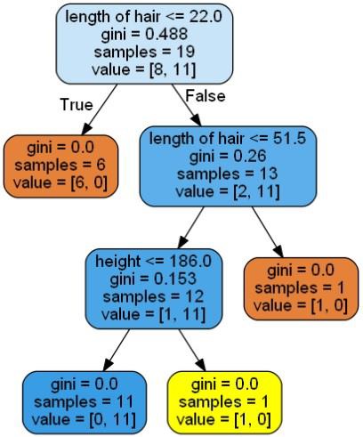
We can change the values of features in prediction to test it.

Random Forest Classifier

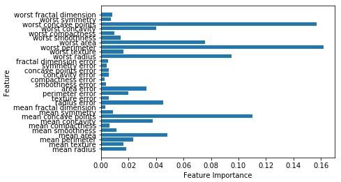
As we know that ensemble methods are the methods which combine machine learning models into a more powerful machine learning model. Random Forest, a collection of decision trees, is one of them. It is better than single decision tree because while retaining the predictive powers it can reduce over-fitting by averaging the results. Here, we are going to implement the random forest model on scikit learn cancer dataset.

Import the necessary packages −

from sklearn.ensemble import RandomForestClassifier
from sklearn.model_selection import train_test_split
from sklearn.datasets import load_breast_cancer
cancer = load_breast_cancer()
import matplotlib.pyplot as plt
import numpy as np

Now, we need to provide the dataset which can be done as follows &minus

cancer = load_breast_cancer()
X_train, X_test, y_train,
y_test = train_test_split(cancer.data, cancer.target, random_state = 0)

After providing the dataset, we need to fit the model which can be done as follows −

forest = RandomForestClassifier(n_estimators = 50, random_state = 0)
forest.fit(X_train,y_train)

Now, get the accuracy on training as well as testing subset: if we will increase the number of estimators then, the accuracy of testing subset would also be increased.

print('Accuracy on the training subset:(:.3f)',format(forest.score(X_train,y_train)))
print('Accuracy on the training subset:(:.3f)',format(forest.score(X_test,y_test)))

Output

Accuracy on the training subset:(:.3f) 1.0
Accuracy on the training subset:(:.3f) 0.965034965034965

Now, like the decision tree, random forest has the feature_importance module which will provide a better view of feature weight than decision tree. It can be plot and visualize as follows −

n_features = cancer.data.shape[1]
plt.barh(range(n_features),forest.feature_importances_, align='center')
plt.yticks(np.arange(n_features),cancer.feature_names)
plt.xlabel('Feature Importance')
plt.ylabel('Feature')
plt.show()

Performance of a classifier

After implementing a machine learning algorithm, we need to find out how effective the model is. The criteria for measuring the effectiveness may be based upon datasets and metric. For evaluating different machine learning algorithms, we can use different performance metrics. For example, suppose if a classifier is used to distinguish between images of different objects, we can use the classification performance metrics such as average accuracy, AUC, etc. In one or other sense, the metric we choose to evaluate our machine learning model is very important because the choice of metrics influences how the performance of a machine learning algorithm is measured and compared. Following are some of the metrics −

Confusion Matrix

Basically it is used for classification problem where the output can be of two or more types of classes. It is the easiest way to measure the performance of a classifier. A confusion matrix is basically a table with two dimensions namely “Actual” and “Predicted”. Both the dimensions have “True Positives (TP)”, “True Negatives (TN)”, “False Positives (FP)”, “False Negatives (FN)”.

In the confusion matrix above, 1 is for positive class and 0 is for negative class.

Following are the terms associated with Confusion matrix −

• True Positives − TPs are the cases when the actual class of data point was 1 and the predicted is also 1.

• True Negatives − TNs are the cases when the actual class of the data point was 0 and the predicted is also 0.

• False Positives − FPs are the cases when the actual class of data point was 0 and the predicted is also 1.

• False Negatives − FNs are the cases when the actual class of the data point was 1 and the predicted is also 0.

Accuracy

The confusion matrix itself is not a performance measure as such but almost all the performance matrices are based on the confusion matrix. One of them is accuracy. In classification problems, it may be defined as the number of correct predictions made by the model over all kinds of predictions made. The formula for calculating the accuracy is as follows −

$$Accuracy = \frac{TP+TN}{TP+FP+FN+TN}$$

Precision

It is mostly used in document retrievals. It may be defined as how many of the returned documents are correct. Following is the formula for calculating the precision −

$$Precision = \frac{TP}{TP+FP}$$

Recall or Sensitivity

It may be defined as how many of the positives do the model return. Following is the formula for calculating the recall/sensitivity of the model −

$$Recall = \frac{TP}{TP+FN}$$

Specificity

It may be defined as how many of the negatives do the model return. It is exactly opposite to recall. Following is the formula for calculating the specificity of the model −

$$Specificity = \frac{TN}{TN+FP}$$

Class Imbalance Problem

Class imbalance is the scenario where the number of observations belonging to one class is significantly lower than those belonging to the other classes. For example, this problem is prominent in the scenario where we need to identify the rare diseases, fraudulent transactions in bank etc.

Example of imbalanced classes

Let us consider an example of fraud detection data set to understand the concept of imbalanced class −

Total observations = 5000
Fraudulent Observations = 50
Non-Fraudulent Observations = 4950
Event Rate = 1%

Solution

Balancing the classes’ acts as a solution to imbalanced classes. The main objective of balancing the classes is to either increase the frequency of the minority class or decrease the frequency of the majority class. Following are the approaches to solve the issue of imbalances classes −

Re-Sampling

Re-sampling is a series of methods used to reconstruct the sample data sets − both training sets and testing sets. Re-sampling is done to improve the accuracy of model. Following are some re-sampling techniques −

• Random Under-Sampling − This technique aims to balance class distribution by randomly eliminating majority class examples. This is done until the majority and minority class instances are balanced out.

Total observations = 5000
Fraudulent Observations = 50
Non-Fraudulent Observations = 4950
Event Rate = 1%

In this case, we are taking 10% samples without replacement from non-fraud instances and then combine them with the fraud instances −

Non-fraudulent observations after random under sampling = 10% of 4950 = 495

Total observations after combining them with fraudulent observations = 50+495 = 545

Hence now, the event rate for new dataset after under sampling = 9%

The main advantage of this technique is that it can reduce run time and improve storage. But on the other side, it can discard useful information while reducing the number of training data samples.

• Random Over-Sampling − This technique aims to balance class distribution by increasing the number of instances in the minority class by replicating them.

Total observations = 5000
Fraudulent Observations = 50
Non-Fraudulent Observations = 4950
Event Rate = 1%

In case we are replicating 50 fraudulent observations 30 times then fraudulent observations after replicating the minority class observations would be 1500. And then total observations in the new data after oversampling would be 4950+1500 = 6450. Hence the event rate for the new data set would be 1500/6450 = 23%.

The main advantage of this method is that there would be no loss of useful information. But on the other hand, it has the increased chances of over-fitting because it replicates the minority class events.

Ensemble Techniques

This methodology basically is used to modify existing classification algorithms to make them appropriate for imbalanced data sets. In this approach we construct several two stage classifier from the original data and then aggregate their predictions. Random forest classifier is an example of ensemble based classifier.