Cross Referencing in Excel 2010

---

Graphic Objects in MS Excel

When you have information spread across several different spreadsheets, it can seem a daunting task to bring all these different sets of data together into one meaningful list or table. This is where the Vlookup function comes into its own.

VLOOKUP

VlookUp searches for a value vertically down for the lookup table. VLOOKUP(lookup_value,table_array,col_index_num,range_lookup) has 4 parameters as below.

• lookup_value − It is the user input. This is the value that the function uses to search on.

• The table_array − It is the area of cells in which the table is located. This includes not only the column being searched on, but the data columns for which you are going to get the values that you need.

• Col_index_num − It is the column of data that contains the answer that you want.

• Range_lookup − It is a TRUE or FALSE value. When set to TRUE, the lookup function gives the closest match to the lookup_value without going over the lookup_value. When set to FALSE, an exact match must be found to the lookup_value or the function will return #N/A. Note, this requires that the column containing the lookup_value be formatted in ascending order.

VLOOKUP Example

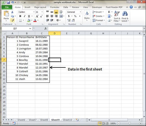
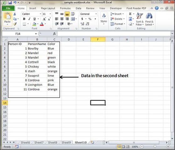
Let's look at a very simple example of cross-referencing two spreadsheets. Each spreadsheet contains information about the same group of people. The first spreadsheet has their dates of birth, and the second shows their favorite color. How do we build a list showing the person's name, their date of birth and their favorite color? VLOOOKUP will help in this case. First of all, let us see data in both the sheets.

This is data in the first sheet

This is data in the second sheet

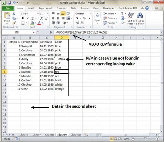
Now for finding the respective favorite color for that person from another sheet we need to vlookup the data. First argument to the VLOOKUP is lookup value (In this case it is person name). Second argument is the table array, which is table in the second sheet from B2 to C11. Third argument to VLOOKUP is Column index num, which is the answer we are looking for. In this case, it is 2 the color column number is 2. The fourth argument is True returning partial match or false returning exact match. After applying VLOOKUP formula it will calculate the color and the results are displayed as below.

As you can see in the above screen-shot that results of VLOOKUP has searched for color in the second sheet table. It has returned #N/A in case where match is not found. In this case, Andy's data is not present in the second sheet so it returned #N/A.