- TensorFlow Tutorial
- TensorFlow - Home
- TensorFlow - Introduction
- TensorFlow - Installation
- Understanding Artificial Intelligence
- Mathematical Foundations
- Machine Learning & Deep Learning
- TensorFlow - Basics
- Convolutional Neural Networks
- Recurrent Neural Networks
- TensorBoard Visualization
- TensorFlow - Word Embedding
- Single Layer Perceptron
- TensorFlow - Linear Regression
- TFLearn and its installation
- CNN and RNN Difference
- TensorFlow - Keras
- TensorFlow - Distributed Computing
- TensorFlow - Exporting
- Multi-Layer Perceptron Learning
- Hidden Layers of Perceptron
- TensorFlow - Optimizers
- TensorFlow - XOR Implementation
- Gradient Descent Optimization
- TensorFlow - Forming Graphs
- Image Recognition using TensorFlow
- Recommendations for Neural Network Training
- TensorFlow Useful Resources
- TensorFlow - Quick Guide
- TensorFlow - Useful Resources
- TensorFlow - Discussion
- Selected Reading
- UPSC IAS Exams Notes
- Developer's Best Practices
- Questions and Answers
- Effective Resume Writing
- HR Interview Questions
- Computer Glossary
- Who is Who
TensorFlow - Multi-Layer Perceptron Learning
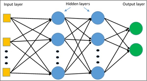
Multi-Layer perceptron defines the most complicated architecture of artificial neural networks. It is substantially formed from multiple layers of perceptron.
The diagrammatic representation of multi-layer perceptron learning is as shown below −

MLP networks are usually used for supervised learning format. A typical learning algorithm for MLP networks is also called back propagation’s algorithm.
Now, we will focus on the implementation with MLP for an image classification problem.
# Import MINST data
from tensorflow.examples.tutorials.mnist import input_data
mnist = input_data.read_data_sets("/tmp/data/", one_hot = True)

import tensorflow as tf
import matplotlib.pyplot as plt

# Parameters
learning_rate = 0.001
training_epochs = 20
batch_size = 100
display_step = 1

# Network Parameters
n_hidden_1 = 256

# 1st layer num features
n_hidden_2 = 256 # 2nd layer num features
n_input = 784 # MNIST data input (img shape: 28*28) n_classes = 10
# MNIST total classes (0-9 digits)

# tf Graph input
x = tf.placeholder("float", [None, n_input])
y = tf.placeholder("float", [None, n_classes])

# weights layer 1
h = tf.Variable(tf.random_normal([n_input, n_hidden_1])) # bias layer 1
bias_layer_1 = tf.Variable(tf.random_normal([n_hidden_1]))
# layer 1 layer_1 = tf.nn.sigmoid(tf.add(tf.matmul(x, h), bias_layer_1))

# weights layer 2
w = tf.Variable(tf.random_normal([n_hidden_1, n_hidden_2]))

# bias layer 2
bias_layer_2 = tf.Variable(tf.random_normal([n_hidden_2]))

# layer 2
layer_2 = tf.nn.sigmoid(tf.add(tf.matmul(layer_1, w), bias_layer_2))

# weights output layer
output = tf.Variable(tf.random_normal([n_hidden_2, n_classes]))

# biar output layer
bias_output = tf.Variable(tf.random_normal([n_classes])) # output layer
output_layer = tf.matmul(layer_2, output) + bias_output

# cost function
cost = tf.reduce_mean(tf.nn.sigmoid_cross_entropy_with_logits(
   logits = output_layer, labels = y))

#cost = tf.reduce_mean(tf.nn.sigmoid_cross_entropy_with_logits(output_layer, y))
# optimizer
optimizer = tf.train.AdamOptimizer(learning_rate = learning_rate).minimize(cost)

# optimizer = tf.train.GradientDescentOptimizer(
   learning_rate = learning_rate).minimize(cost)

# Plot settings
avg_set = []
epoch_set = []

# Initializing the variables
init = tf.global_variables_initializer()

# Launch the graph
with tf.Session() as sess:
   sess.run(init)

   # Training cycle
   for epoch in range(training_epochs):
      avg_cost = 0.
      total_batch = int(mnist.train.num_examples / batch_size)

      # Loop over all batches
      for i in range(total_batch):
         batch_xs, batch_ys = mnist.train.next_batch(batch_size)
         # Fit training using batch data sess.run(optimizer, feed_dict = {
            x: batch_xs, y: batch_ys})
         # Compute average loss
         avg_cost += sess.run(cost, feed_dict = {x: batch_xs, y: batch_ys}) / total_batch
      # Display logs per epoch step
      if epoch % display_step == 0:
         print
         Epoch:", '%04d' % (epoch + 1), "cost=", "{:.9f}".format(avg_cost)
      avg_set.append(avg_cost)
      epoch_set.append(epoch + 1)
   print
   "Training phase finished"

   plt.plot(epoch_set, avg_set, 'o', label = 'MLP Training phase')
   plt.ylabel('cost')
   plt.xlabel('epoch')
   plt.legend()
   plt.show()

   # Test model
   correct_prediction = tf.equal(tf.argmax(output_layer, 1), tf.argmax(y, 1))

   # Calculate accuracy
   accuracy = tf.reduce_mean(tf.cast(correct_prediction, "float"))
   print
   "Model Accuracy:", accuracy.eval({x: mnist.test.images, y: mnist.test.labels})
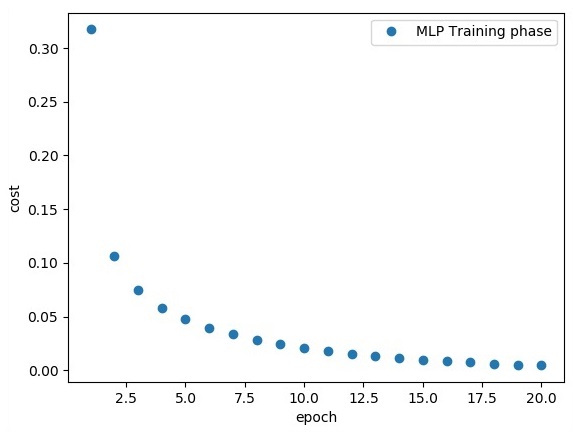
The above line of code generates the following output −

Advertisements